by Mauro Serralvo, founder at BrinPage.

On this page, I will try to explain the basic technical concepts of AI so that even a non-technical person can understand them. Understanding artificial intelligence begins with clarifying what the term actually encompasses. At its core, AI refers to a branch of computer science dedicated to creating systems that can perform tasks typically associated with human intelligence—such as reasoning, learning from data, recognizing patterns, and making informed decisions. Unlike traditional software, which operates based on explicitly programmed rules, AI systems are designed to improve through experience, adjusting their internal models based on the data they process.

One of the key building blocks of modern AI is the neural network—a computational model loosely inspired by the way biological neurons interact in the human brain. When structured in layers, these networks can learn to identify complex patterns and relationships within data. The purpose of this document is to provide a foundational overview of the core theoretical principles behind neural networks, including how they are constructed, trained, and evaluated in practical applications.

Neural networks are computational models loosely inspired by the structure and function of the human brain. They consist of layers of interconnected units known as neurons, each of which processes input signals, applies an activation function, and generates an output. By adjusting connection weights and bias terms during training, these networks are able to model and recognize complex patterns within data. Neural networks are central to deep learning and have enabled significant advances across various domains of AI.

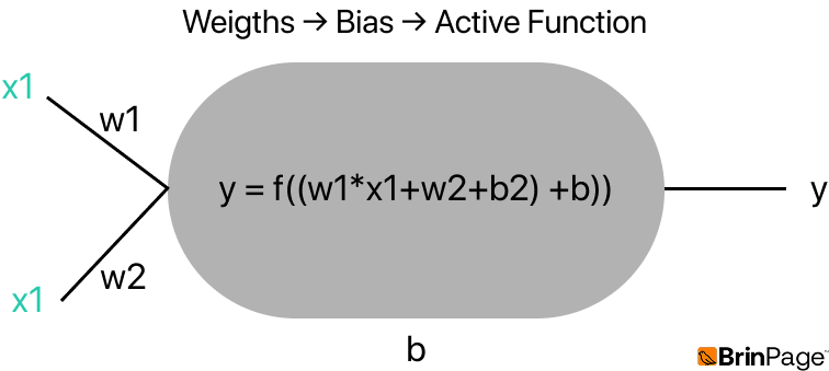
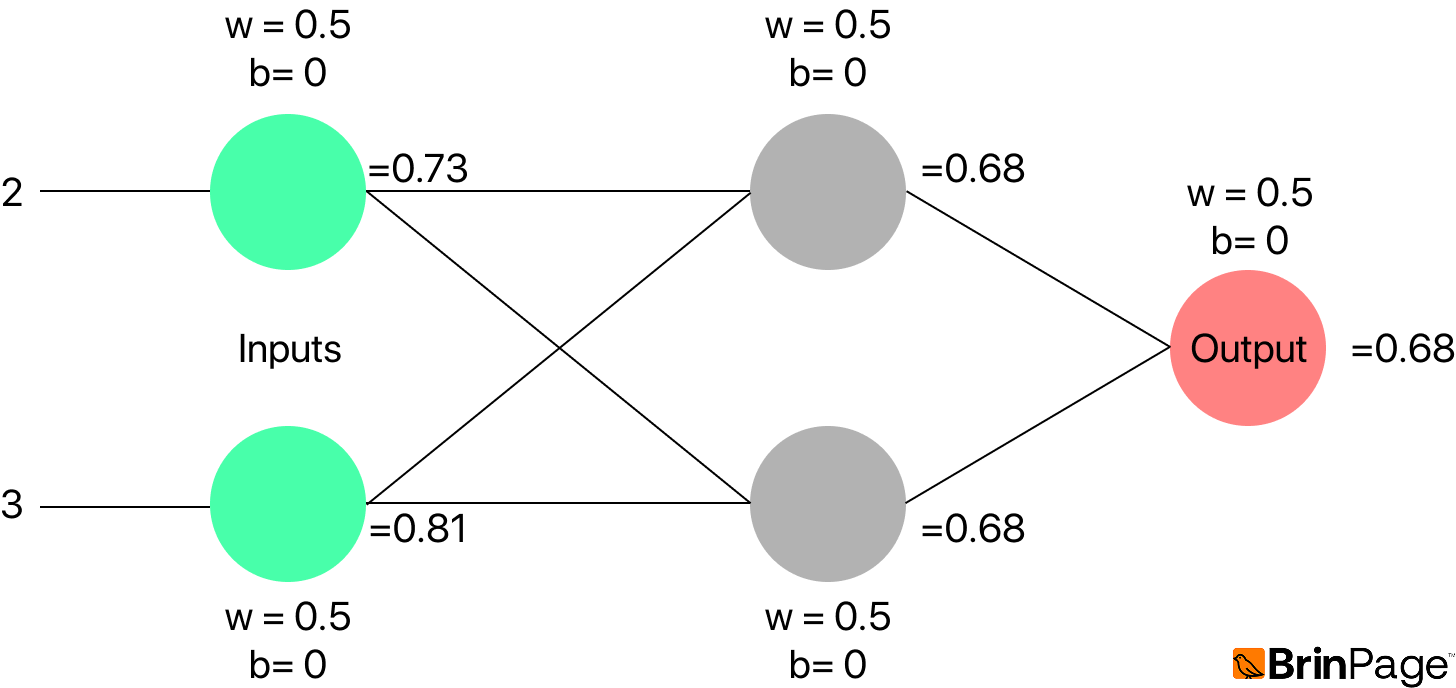
Consider a simple example with two inputs: x₁ = 2 and x₂ = 3, with associated weights w₁ = 0.5 and w₂ = 0.5. The bias is set to b = 0, and the activation function used is the sigmoid function.
The neuron computes:
y = sigmoid(x₁ ⋅ w₁ + x₂ ⋅ w₂ + b)
Substituting the values:
y = sigmoid(2 ⋅ 0.5 + 3 ⋅ 0.5 + 0) = sigmoid(2.5) ≈ 0.92
This example illustrates how weights and biases influence the output, while the activation function introduces non-linearity—allowing the model to capture more complex patterns than a linear function could.

Here, the weights and bias directly influence the output, and the activation function introduces non-linearity. Without non-linear activation, the network could only learn simple linear relationships.

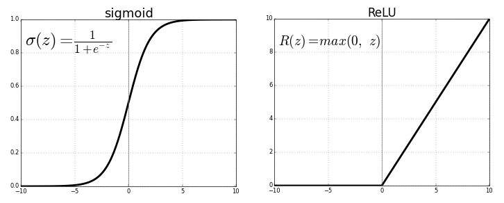
The most common activation functions are:
- Sigmoid – compresses outputs between 0 and 1.
- ReLU (Rectified Linear Unit) – outputs 0 for negative inputs and passes positive values unchanged.

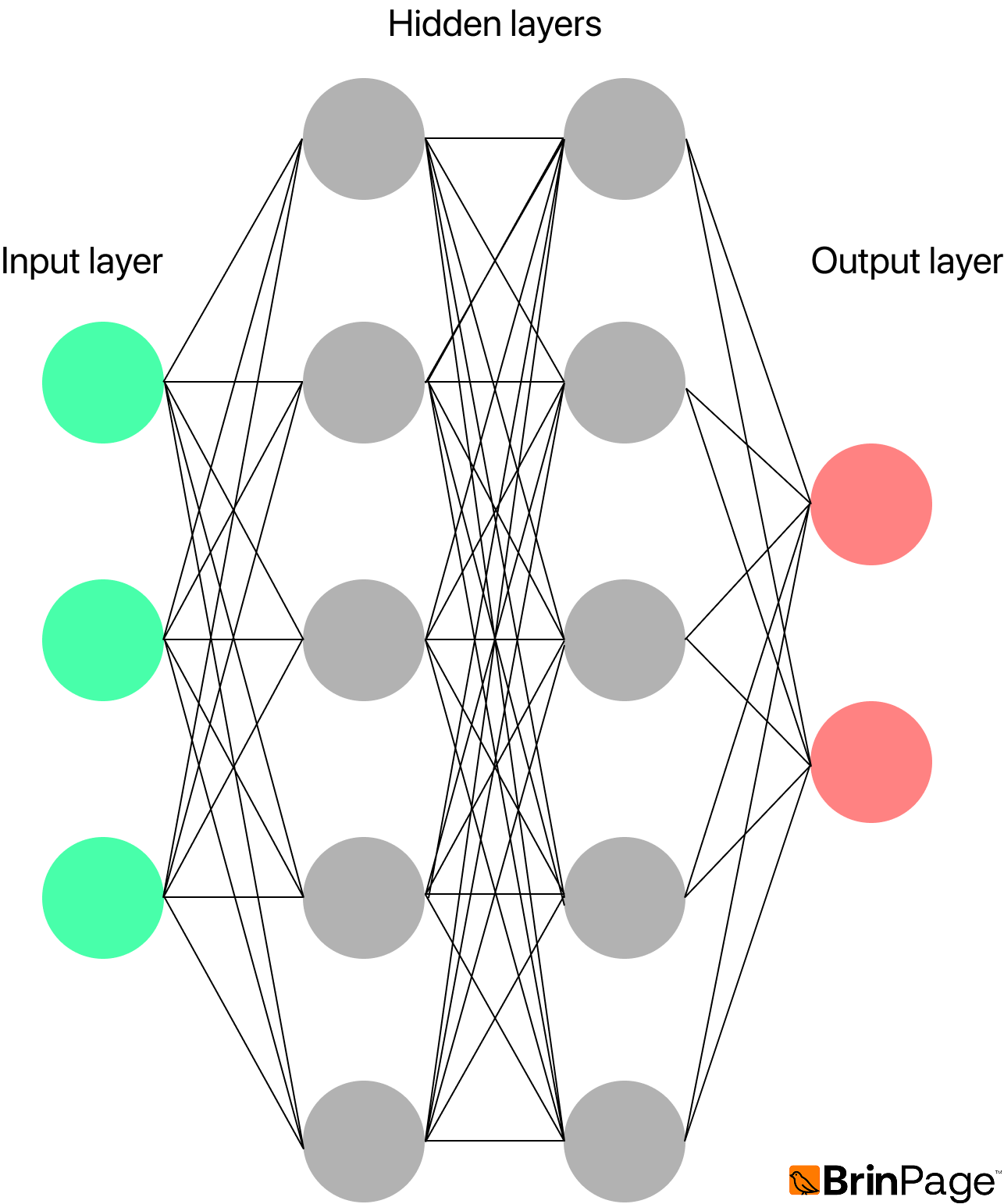
When neurons are organized into multiple layers, the network is able to learn increasingly abstract representations of the input. Typically, early layers detect low-level features such as edges or lines; intermediate (hidden) layers combine these into more complex patterns like curves or intersections; and the final layers capture high-level concepts, such as identifying that an image represents the digit “5”.

This hierarchy of feature detection is the basis of deep learning. By training on millions of labeled examples (e.g., handwritten digits 0–9), the network adjusts its weights and biases automatically to minimize prediction errors.

Training a neural network involves feeding it a large set of input-output pairs, allowing the model to learn the underlying relationships. For example, in a simple addition task, the dataset might include pairs like (1,1) → 2, (1,2) → 3, and so on. The quality of this dataset is critical—it must be accurate, consistent in format, and diverse enough to promote generalization.

The dataset must be: Accurate (labels must be correct), Consistent (uniform format), Diverse (covering enough variations to generalize).

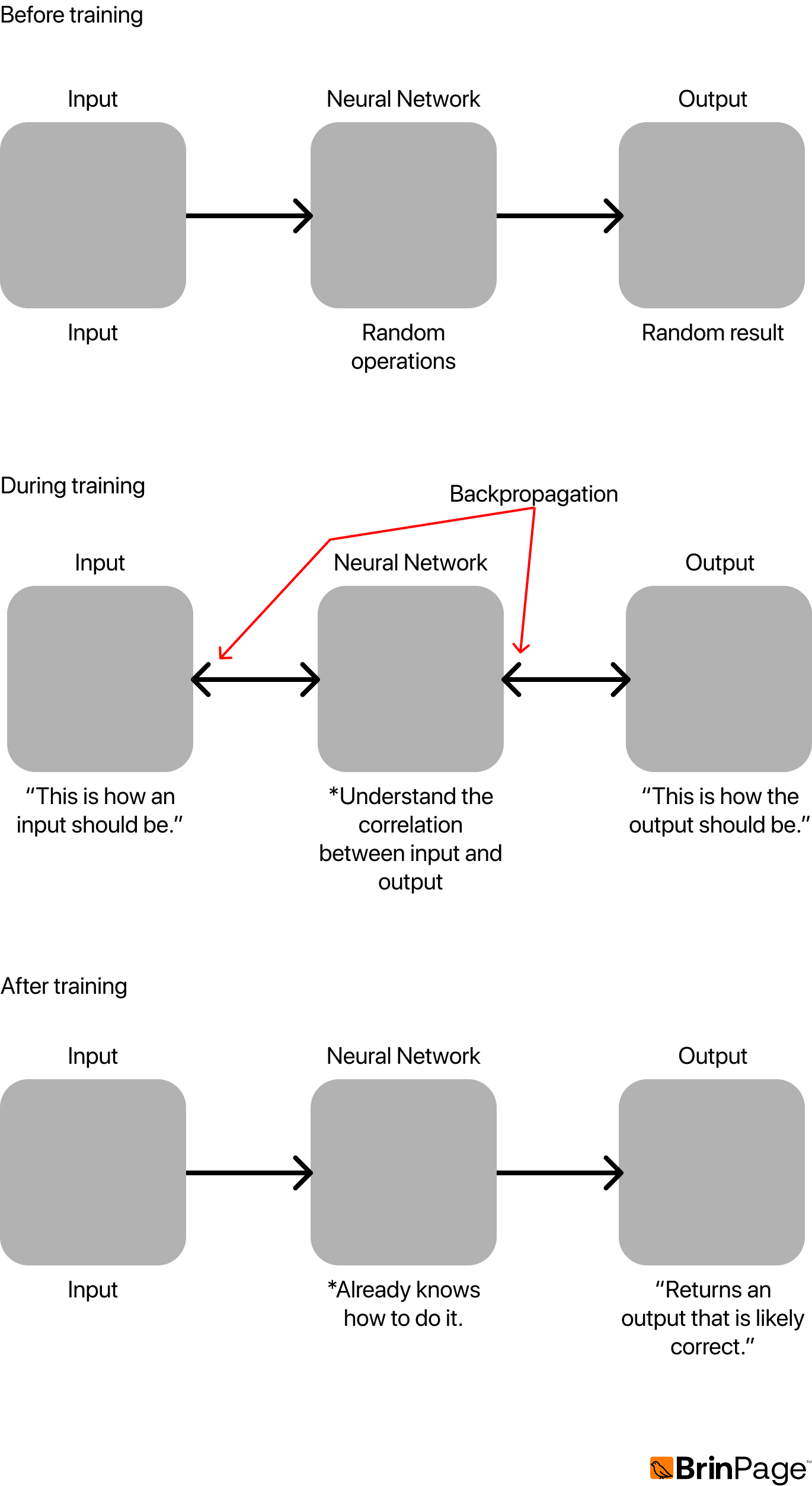
The key mechanism in training is backpropagation. If the network produces the wrong output, we calculate the error and propagate it backward through the network. This process updates the weights and biases in order to reduce future errors.

Training uses batches of data, where each batch contains multiple samples. Small models may be trained on hundreds of samples, while large models require millions.

To measure how well the model performs, we compute a loss function, which quantifies the difference between the predicted output and the expected output.

A common loss function is Mean Squared Error (MSE):

In this context, y_i represents the expected output, while ŷ_i is the predicted output. The variable N stands for the total number of predictions.

A lower loss indicates better accuracy, whereas a higher loss suggests poorer model performance.

For example, if the model starts with a Mean Squared Error (MSE) of 2.5 and we make an incorrect adjustment to the bias b₁, the MSE might increase to 2.7. However, if we adjust a different bias, say b₃, the MSE could improve to 2.0.

A common loss function is Mean Squared Error (MSE):

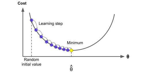
To minimize the loss, we apply gradient descent. This involves computing the partial derivatives of the loss with respect to each weight and bias, allowing us to determine how each parameter should be adjusted.

When the derivative is positive, it indicates the weight should be decreased. Conversely, if the derivative is negative, the weight should be increased.

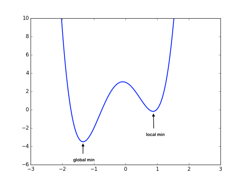
These adjustments are scaled by the learning rate, which controls how large each step is. A rate that’s too small can lead to slow learning or cause the model to get stuck in a local minimum. On the other hand, a rate that’s too large can make training unstable and may overshoot the optimal point.

Ultimately, the goal is to reach the global minimum of the loss function, where the model performs at its best.

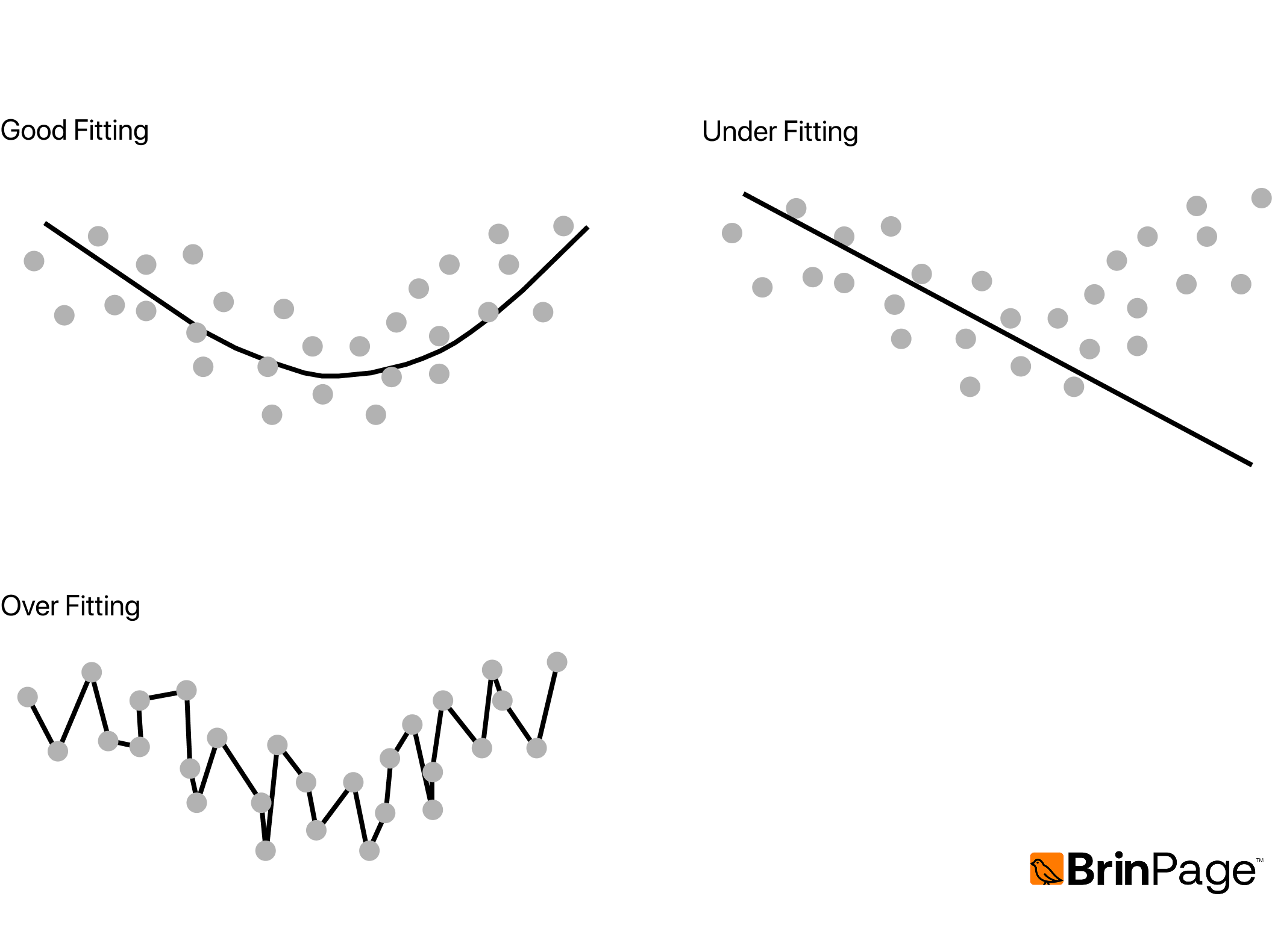
Fitting describes how well a model has learned from the training data.

When a model is underfitting, it's too simple to capture meaningful patterns — it struggles with both the training data and unseen data, leading to poor performance overall.

On the other hand, overfitting occurs when the model learns the training data too well, even memorizing noise. It performs very well on the training set but fails to generalize to new data.

Ideally, we aim for good fitting, where the model captures the true structure of the data and generalizes effectively, balancing learning and flexibility without overreacting to noise.

The way data is represented has a significant impact on how effectively a model learns. Both features (inputs) and labels (expected outputs) must be structured in a way that allows the neural network to identify and extract meaningful patterns.

For example, if the input feature is the square meters of a house and the label is its price, then—given enough diverse training samples—the model can learn the relationship and predict prices for house sizes it has never seen before.

In practice, data is stored in tensors, which are multidimensional arrays. Tensors provide the structure needed to represent complex data in a way that neural networks can process efficiently.

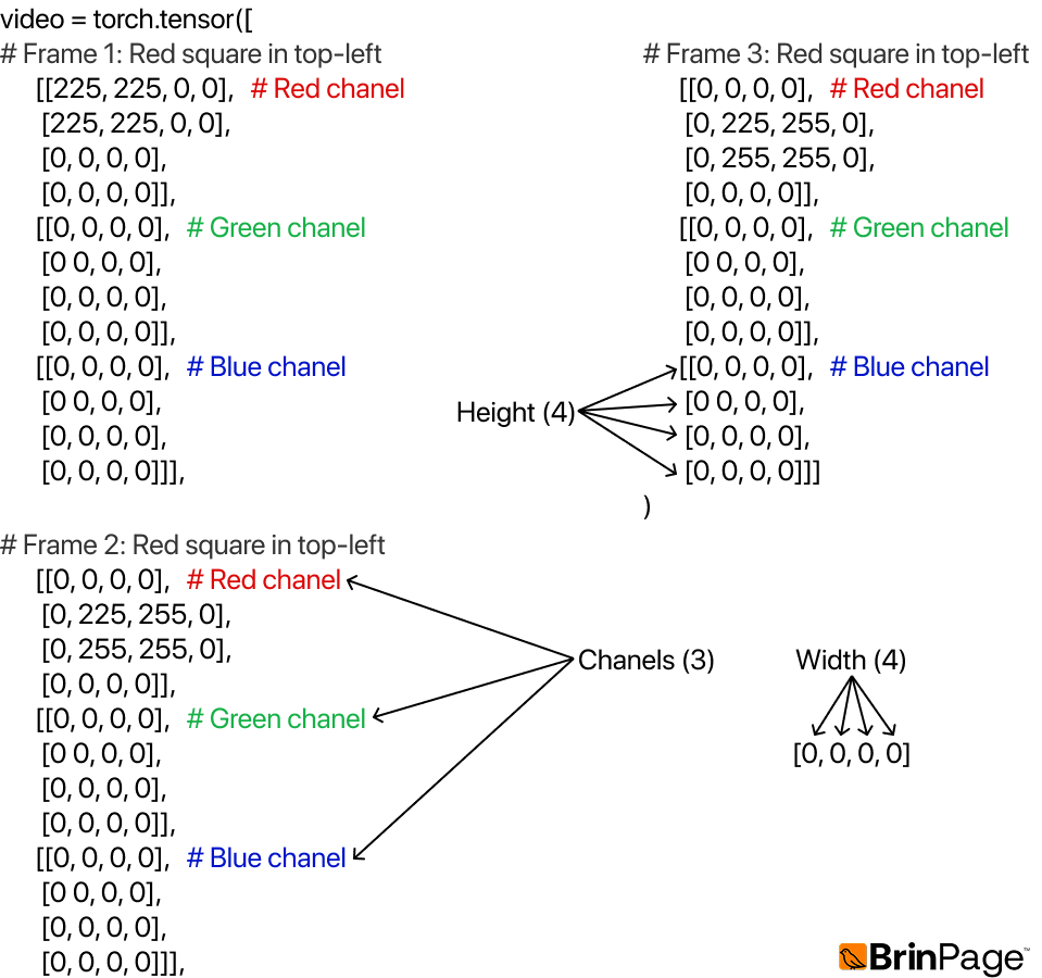
By adding more dimensions to a tensor, we can represent richer forms of data. For instance, a video can be represented as a 4D tensor, where each axis corresponds to the number of frames, the color channels (RGB), the height, and the width of the image. This transformation of raw information into a tensor-based format is known as encoding.

Video example = [frames=3, channels=3, height=4, width=4]

The image above shows how a simple video with three frames can be broken down visually into separate color channels (red, green, and blue). Each frame is essentially a small image composed of pixel values across these channels.

In the next step, this visual structure can be encoded into numerical arrays (tensors), where every pixel value is stored as a number. This is illustrated in the following diagram, which shows the underlying array representation of the same video data.

When building a neural network, the input layer must be designed to match the size and shape of the input tensor, while the output layer should be structured according to the size and shape of the expected results.

This section has introduced the fundamental concepts underpinning modern AI systems: neural networks, training algorithms, loss functions, optimization strategies, model fitting, and data representation. These elements form the basis for the models we develop at BrinPage. A solid understanding of how these systems learn and adapt is essential for designing AI that moves beyond rule-based software and creates real-world impact.

In the next part of the documentation, we move from theory to practice, presenting BirdMind v0, our first code generation model, and explaining how these concepts are applied in its design and implementation.

Brinpage Software ©2025